Definitions
Container: a collection of software components and artifacts. Component: (software) a single piece of software, e.g., an executable, shared library, or firmware blob. Artefact: (not software) any non-software file or blob that exists within a container. Environment: a static or dynamic configuration of components and artefacts. An environment determines which components within a container to load, which component is run first, and/or which components run at all. It may contain a component loader, that is, a component that can be used to execute other components. It may provide a mechanism to configure components such that one or more components within a given environment may interact with each other. It may also provide a mechanism for restricting how components interact with each other, with artefacts (e.g., via filesystem permissions), and with the outside world. Entry-point: a location within a component that execution can start from, e.g., the main function in an executable component, or one of the exported functions within a shared library. It may or may not be advertised to other components or the environment’s program loader.Intra-component Reachability
A software component contains one or more functions, and these functions may call each other and the functions of other components, depending on the properties of the environment. A function can be decomposed into so-called basic blocks, which are sequences of one or more machine code instructions that are always terminated by a control-flow altering instruction, e.g., an instruction that causes a branch, call, interrupt, or exception. Each instruction within a basic block can be considered a program point. The reachability of a program point, given the definition of a basic block, is therefore equivalent to the reachability of the basic block containing it.Control-flow properties
We can model the control transfers between each basic block within a component by representing the component as one or more inter-procedural control-flow graphs (ICFGs). The vertices of such graphs are basic blocks and the edges are control-flow operations. These graphs statically model how control transitions between both functions and basic blocks by different control-flow altering operations. Multiple graphs may be required to represent a single component, for example, where a component contains so-called dead or unreachable code, when it is a library of related functionality, or when it is not possible to completely recover the target of one or more indirect branches or calls.Data-flow properties
Given a control-flow graph representation of a component, we can model its data-flow, i.e., how data moves between different program variables, and the properties of the values held in those variables at different points during execution. Using an abstract interpretation technique such as Value Set Analysis (VSA), or a data-flow technique such as constant propagation, we can compute an approximation of the values a given variable can hold at a given point. With this information, we can perform two operations on the ICFGs:- Update them by adding new control-flow edges when we are able to infer the possible values a variable holds when used as the target of an indirect branch or call instruction.
- Update them by removing control-flow edges when we are able to infer that the value of a variable used to determine if a branch is taken or not may only have a single value.
Code cross-reference properties
The information described above also allows us to build a second graph-based model of a component based on the direct and indirect targets of its load operations. We refer to such a graph as the code cross-reference graph. This graph may be overlayed onto the ICFGs of the component to model their potential dependencies.Computing reachability
To compute the reachability of one or more program points within a component, we perform the following procedure:- Construct a set of initial ICFGs for the component. We may use techniques from the literature, for example, recursive descent disassembly, linear disassembly, or a combination/variation of one or both.
- Perform data-flow analysis or abstract interpretation (as described above) of the ICFGs to determine potential unreachable or dead-code, and missing edges and/or basic blocks. This results in a number of data-flow graphs (DFGs) representing the relationships between variables and program points within each ICFG.
- Construct a code cross-reference graph of the resulting ICFGs. That is we construct a graph with vertices representing basic blocks and edges representing load operations referencing program points. The load operations may also represent transitive relations, for example, if we have a reference from block A to a data structure D and data structure D refers to block B, then we produce an edge from block A to B.
- Identify entry-points of the components based on the ICFGs. This process will vary depending on the platform the component is from and the type of the component. We provide some examples: A shared library will export a number of functions that can be called by other components–we will consider each of these a viable entry-point. An executable will export a start or main function–we will consider this function a viable entry-point. A UEFI driver/module may export functionality via a protocol or interface; they may also register functions to be called upon particular events. We consider all functions exported using these mechanisms as viable entry-points. For firmware that contain an Interrupt Vector Table (IVT), we consider the defined Interrupt Service Routines (ISRs) as viable entry-points.
- Given the set of entry-points, ICFGs, and program locations we wish to determine the reachability of, we treat reachability as a general reachability problem, and check if there exists a path from any identified entry-point to each program point. In some cases, we may perform a second heavier analysis of each path to provide a reachability proof. This proof is constructed by symbolically executing the by symbolically executing the path.
- Given the set of reachable program locations, we classify the reachability of each location by the type of entry-point(s) used to reach it (see the next section).
- For program locations that are not reachable from any identified entry-points, we perform a second analysis which checks for paths in the graph derived from merging the ICFGs and code cross-reference graph.
- For program locations that are still considered unreachable at this point, we label their reachability as undetermined.
Classifying reachability (from high to low risk)
Direct reachability: this covers the most obvious kind of reachability and is used if there exists a path from the original entry-point (e.g., main or start function) of the component analysed to the vulnerable program location. Exported reachability: this covers indirect reachability, for example, for shared libraries, we assume exported functions are viable entry-points, and if a finding is reachable from an exported function, then we report it as “exported” reachability. We also use this classification for identified SMI handlers, functions in registered protocol interfaces and PPIs, in UEFI modules/drivers. Referenced reachability: this covers cases where a vulnerable point is reachable because it is referenced by code that is reachable by direct or exported reachability, but we are unable to determine the exact reachability statically. Undetermined reachability: this covers all cases where we are unable to determine reachability statically. In addition to a classification of reachability we compute “trace evidence”, i.e., one or more paths through the ICFG to show that a given point is reachable, and metrics quantifying the difficulty of reaching a given program point via each of those paths. These metrics include quantifications of branching/sub-call graph complexity, distance metrics computed on the paths, number of possible paths that allow a given point to be considered reachable.Extended reachability properties
Given a component does not operate in isolation of its environment, it is desirable to contextualise the reachability characteristics of a given vulnerable location with respect to properties we are able to infer about the environment it will be executed within. This leads us to the notions of inter-component reachability and environment-aware reachability.Inter-component reachability
Similar to how we construct the control-flow graphs of a single component, by considering the exported functions of each component, and “external” functions called by each component, we can build an “inter-component call-graph” between components representing inter-component reachability. The vertices of the graph are components and the edges are exported functions. By checking for the existence of paths within this graph, we associate each of a component’s entry-points with a measure of viability to provide a more granular risk measurement. Concretely, F is a viable (exported) entry-point if we find a component A that calls the exported function F from component B. The above approach can be extended to take into account various platform specifics, for example, Linux-like platforms provide a mechanism to load a shared library at runtime (dlopen) and resolve function symbols (dlsym). In some cases, it is possible to identify such behaviour statically, and the inter-component call-graph can be modified to take this into account.Environment-aware reachability
Recall that within an execution environment we have both artefacts and software components. While artefacts may be regular files, they may also serve to configure the runtime properties of the environment. For example, in an embedded Linux environment, we may have one or more boot scripts that determine which software components will be loaded and executed during the initialisation of the environment. This list of components along with any later stage component-specific configuration files (artefacts), will determine the set of components that can run. While we may not be able to completely determine this set statically, we may approximate it, and we can use this information to mark the viability of all components’ entry-points within the inter-component call-graph, allowing for even finer-grained risk assessment. Other examples of how environment restrictions can be taken into account when determining component entry-point viability are:- A docker container’s “entry-point”–a configuration key associated with a docker container that determines which program or script to execute when the container is launched.
- The second-stage payload blob and associated program location specified by a boot-loader’s configuration.
Reachability use-cases
As noted in the introduction to this document, reachability is generally considered a reasonable proxy for assessing the ease of exploitability of a particular vulnerability or whether the vulnerability is exploitable at all. When used in this context, reachability can be considered a complementary metric to existing industry standard vulnerability severity and exploitability metrics, such as CVSS, EPSS, SSVC, and so on. We foresee reachability being used for the following tasks:- Triage prioritization, i.e., the priority in which a given vulnerability should be assessed–high risk first, low risk last.
- Remediation prioritisation, i.e., the priority in which a given vulnerability should be patched or fixed.
- Risk assessment of 3rd-party components in the context of a larger product or code-base, i.e., how much additional risk does introducing a component with a known vulnerability with a given reachability profile introduce?.
- As a risk reweighting factor, i.e., when reachability is computed on an environmental or inter-component level, it may be used to rescore the impact or severity of a known vulnerability (i.e., its CVSS score) considered in the context of where the vulnerability exists within a wider product or code-base.
Call-graph Reachability
We will introduce support for call-graph reachability metrics in the coming week for all supported platforms where we perform in-depth code analysis to detect issues. These metrics will report how a given finding (vulnerability) can be reached within a given binary. We classify call-graph reachability based on the kind of “entrypoint” a given finding is reachable from. These entry points cover:- Direct reachability–this covers the most obvious kind of reachability and is reported if there exists a path in the call graph from the original entrypoint of the binary analyzed to the finding location. We refer to this kind of reachability as “entrypoint” reachability.
- Exported reachability–this covers indirect reachability, for example, for BMC firmware which contains shared libraries, we assume exported functions are viable entry points, and if a finding is reachable from an exported function, then we report it as “exported” reachability. For UEFI, we consider identified SMI handlers, functions in registered protocol interfaces and PPIs, and so on, as if they are exports.
- Referenced reachability–this covers cases where we believe a finding is reachable because it is referenced from code that is reachable by direct or exported reachability, but we are unable to determine the exact reachability statically.
- Undetermined reachability–this covers all cases where we are unable to determine reachability statically.
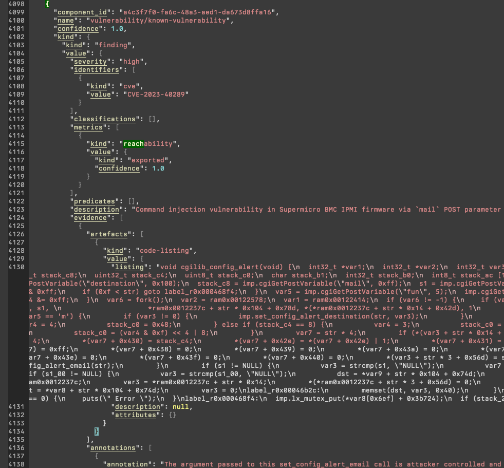
Example: BMC (known vulnerability, CVE-2023-40289; ARM 32-bit)
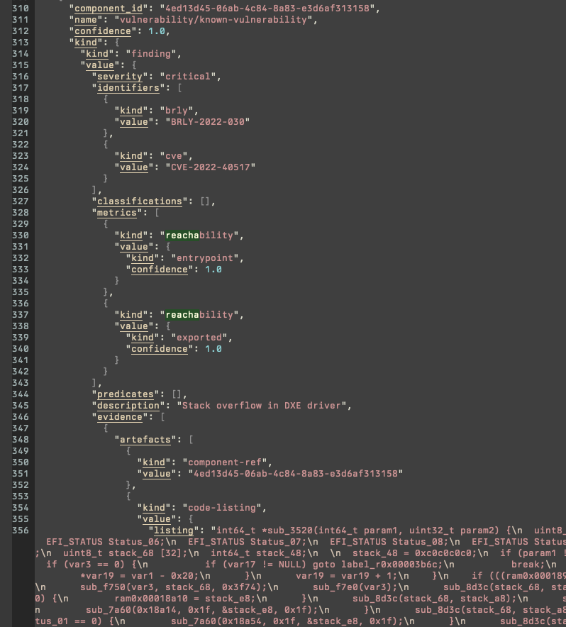
Example: UEFI (known vulnerability, CVE-2022-40517, Shuttle; x86-64)
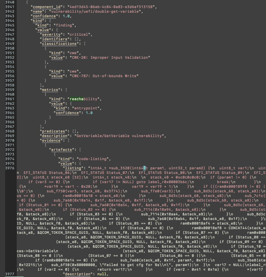
Example: UEFI (unknown vulnerability, double GetVariable, QCOM; AArch64)
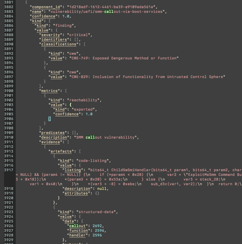
Example: UEFI (unknown vulnerability, SMM callout; x86-64)